I came across this very practical online course Introduction to Machine Learning for Coders(http://course18.fast.ai/ml) on Twitter. I watched the first 7 lessons and enjoyed it so far. I was able to see how Jeremy approach these problems and got many tips and tricks along the way.
The part I watched is focused on Random Forest (RF). I decide to write down some notes for future reference.
1. feature engineer
1.1 categorical -> numerical/one-hot encoding
RF doesn’t handle ‘character’ columns, we need to make them as numbers.
key commands:
# categorical to numerical
pd.Categorical(col).codes
# dummy
df = pd.get_dummies(df, dummy_na=True)
def numericalize(df, col, name, max_n_cat):
    """ Changes the column col from a categorical type to it's integer codes.
    ---------
    >>> df = pd.DataFrame({'col1' : [1, 2, 3], 'col2' : ['a', 'b', 'a']})
    >>> df
       col1 col2
    0     1    a
    1     2    b
    2     3    a
    >>> numericalize(df, df['col2'], 'col3', None)
       col1 col2 col3
    0     1    a    1
    1     2    b    2
    2     3    a    1
    """
    if not is_numeric_dtype(col) and ( max_n_cat is None or len(col.cat.categories)>max_n_cat):
        df[name] = pd.Categorical(col).codes+1
1.2 missing -> fill with mean/median + add column of missingness indicator
We often see missing value, and missingness is usually useful information
key commands:
# indicator
pd.isnull(col)
# fill na
col.fillna(filler)
def fix_missing(df, col, name, na_dict):
    """ Fill missing data in a column of df with the median, and add a {name}_na column
    which specifies if the data was missing.
    ---------
    >>> df = pd.DataFrame({'col1' : [1, np.NaN, 3], 'col2' : [5, 2, 2]})
    >>> df
       col1 col2
    0     1    5
    1   nan    2
    2     3    2
    >>> fix_missing(df, df['col1'], 'col1', {})
    >>> df
       col1 col2 col1_na
    0     1    5   False
    1     2    2    True
    2     3    2   False
    >>> df = pd.DataFrame({'col1' : [1, np.NaN, 3], 'col2' : [5, 2, 2]})
    >>> df
       col1 col2
    0     1    5
    1   nan    2
    2     3    2
    >>> fix_missing(df, df['col2'], 'col2', {})
    >>> df
       col1 col2
    0     1    5
    1   nan    2
    2     3    2
    >>> df = pd.DataFrame({'col1' : [1, np.NaN, 3], 'col2' : [5, 2, 2]})
    >>> df
       col1 col2
    0     1    5
    1   nan    2
    2     3    2
    >>> fix_missing(df, df['col1'], 'col1', {'col1' : 500})
    >>> df
       col1 col2 col1_na
    0     1    5   False
    1   500    2    True
    2     3    2   False
    """
    if is_numeric_dtype(col):
        if pd.isnull(col).sum() or (name in na_dict):
            df[name+'_na'] = pd.isnull(col)  # key
            filler = na_dict[name] if name in na_dict else col.median() # indicator of na
            df[name] = col.fillna(filler)
            na_dict[name] = filler # replace
    return na_dict
1.3 convert date columns
Usually date itself is useless to models, we need to process those: e.g. year, month, week, day of week …
To do that, we can make use of pandas’ datetime data type.
When read into data, specify which column is date, or, convert that column to datetime.
df_raw = pd.read_csv(f'{PATH}Train.csv', low_memory=False,parse_dates=["saledate"])

pd.to_datetime(fld)
import re
def add_datepart(df, fldname, drop=True):
    fld = df[fldname]
    if not np.issubdtype(fld.dtype, np.datetime64):
        df[fldname] = fld = pd.to_datetime(fld,
                                     infer_datetime_format=True)
    targ_pre = re.sub('[Dd]ate$', '', fldname)
    for n in ('Year', 'Month', 'Week', 'Day', 'Dayofweek',
            'Dayofyear', 'Is_month_end', 'Is_month_start',
            'Is_quarter_end', 'Is_quarter_start', 'Is_year_end',
            'Is_year_start'):
        df[targ_pre+n] = getattr(fld.dt,n.lower())
    df[targ_pre+'Elapsed'] = fld.astype(np.int64) // 10**9
    if drop: df.drop(fldname, axis=1, inplace=True)  # drop original col
2. ran RF
Always have training, validation, testing data.
- make sure validation similar to testing
If we are doing forecasting job, don’t random select validation: e.g. use the last 2 weeks
def split_vals(a,n): return a[:n].copy(), a[n:].copy()
n_valid = 12000  # same as Kaggle's test set size
n_trn = len(df)-n_valid
raw_train, raw_valid = split_vals(df_raw, n_trn)
X_train, X_valid = split_vals(df, n_trn)
y_train, y_valid = split_vals(y, n_trn)
X_train.shape, y_train.shape, X_valid.shape
a nice way to summarize results
def rmse(x,y): return math.sqrt(((x-y)**2).mean())
def print_score(m):
    res = [rmse(m.predict(X_train), y_train),
           rmse(m.predict(X_valid), y_valid),
           m.score(X_train, y_train), m.score(X_valid, y_valid)]
    if hasattr(m, 'oob_score_'): res.append(m.oob_score_)
    print(res)
m = RandomForestRegressor(n_jobs=-1)
%time m.fit(X_train, y_train)
print_score(m)
- OOB: usually worse than using validation dataset (since less trees was used to train these data)
From https://medium.com/@hiromi_suenaga/machine-learning-1-lesson-5-df45f0c99618
“So the OOB score gives us something which is pretty similar to the validation score, but on average it’s a little less good. Why? Because every row is going to be using a subset of the trees to make its prediction, and with less trees, we know we get a less accurate prediction. “
- recommended way: use validation to get a good model, then combine train + validation as a dataset to retrain
3. confidence interval
We can get confidence interval for our predictions: for 1 row, make prediction using different trees, summarize these predictions
m = RandomForestRegressor(n_estimators = 40, min_samples_leaf = 3, max_features = 0.5, n_jobs = -1, oob_score = True)
m.fit(X_train,y_train)
preds = np.stack([t.predict(X_valid) for t in m.estimators_]) # this is serial

np.mean(preds[:,0])
np.std(preds[:,0])
4. feature importance
This is something we want really want to see: we usually not care that much about prediction, but to get insights about it.
How to get feature importance?
No need to change the model we get. Simply, we take 1 column, shuffle values in this col, use the model to make predictions, calculate RMSE_shuffle.
Compare to original “real” RMSE, how much changed? That’s feature importance
def rf_feat_importance(m, df):
	"""
	usage:
	fi = rf_feat_importance(m, df_trn); fi[:10]
	# line plot: x axis is cols, y axis is importance
	fi.plot('cols', 'imp', figsize=(10,6), legend=False);
	# bar plot show top 30 features
	def plot_fi(fi): return fi.plot('cols', 'imp', 'barh', figsize=(12,7), legend=False)
	plot_fi(fi[:30]);
	"""
    return pd.DataFrame({'cols':df.columns, 'imp':m.feature_importances_}
                       ).sort_values('imp', ascending=False)
5. remove redundant features
This is really new to me: I haven’t down any filtering like this to reduce redundancy.
There are 2 ways to drop columns
1) set a hard threshold (e.g. imp > 0.5)
fi = rf_feat_importance(m, df_trn); fi[:10]

## downsize happening!

to_keep = fi[fi.imp>0.005].cols; len(to_keep)

df_keep = df_trn[to_keep].copy()
X_train, X_valid = split_vals(df_keep, n_trn)
2) keep 1 of each cluster: we do a hierarchical cluster of features, see the ones in one cluster, get the change in prediction if mess up with that column to decide which ones to drop.
from scipy.cluster import hierarchy as hc

import scipy

corr = np.round(scipy.stats.spearmanr(df_keep).correlation,4)
corr_condensed = hc.distance.squareform(1-corr)
z = hc.linkage(corr_condensed, method = 'average')

fig = plt.figure(figsize=(16,10))
dendrogram = hc.dendrogram(z,labels=df_keep.columns,orientation='left',left_font_size =16)
plt.show()


def get_oob(df):
    m = RandomForestRegressor(n_estimators=30, min_samples_leaf=5, max_features=0.6, n_jobs=-1, oob_score=True)
    x, _ = split_vals(df, n_trn)
    m.fit(x, y_train)
    return m.oob_score_

# look at plot and remove highly related features

for c in ('saleYear', 'saleElapsed', 'fiModelDesc', 'fiBaseModel', 'Grouser_Tracks', 'Coupler_System'):
    print(c, get_oob(df_keep.drop(c, axis=1)))

# It looks like we can try one from each group for removal. Let's see what that does.
to_drop = ['saleYear', 'fiBaseModel', 'Grouser_Tracks']
get_oob(df_keep.drop(to_drop, axis=1))

df_keep.drop(to_drop, axis=1, inplace=True)
X_train, X_valid = split_vals(df_keep, n_trn)
6. partial dependence plot
1D partial dependence plot feels like the coefficients in linear model: fix other variables, how changing this variable will change the outcome.
How do we get there? Say we want to know the partial dependence on ‘Year’, we fix everything else constant in the X matrix, just change ‘Year’ column to ‘1960’, then we average all values got from model taking this modified X as input, we get a point on scatterplot: x = 1960, y = mean().
This is from sklearn documentation: “ PDPs with two target features show the interactions among the two features. For example, the two-variable PDP in the above figure shows the dependence of median house price on joint values of house age and average occupants per household. We can clearly see an interaction between the two features: for an average occupancy greater than two, the house price is nearly independent of the house age, whereas for values less than 2 there is a strong dependence on age.
The sklearn.inspection module provides a convenience function plot_partial_dependence to create one-way and two-way partial dependence plots. In the below example we show how to create a grid of partial dependence plots: two one-way PDPs for the features 0 and 1 and a two-way PDP between the two features:”
from sklearn.datasets import make_hastie_10_2
from sklearn.ensemble import GradientBoostingClassifier
from sklearn.inspection import plot_partial_dependence

X, y = make_hastie_10_2(random_state=0)
clf = GradientBoostingClassifier(n_estimators=100, learning_rate=1.0,max_depth=1, random_state=0).fit(X, y)
features = [0, 1, (0, 1)]
plot_partial_dependence(clf, X, features)
7. tree interpreter
I’ve never heard of this one before.
The idea is: this tree interpreter is for feature importance for a particular observation (row).
We said you mainly use that for a row.
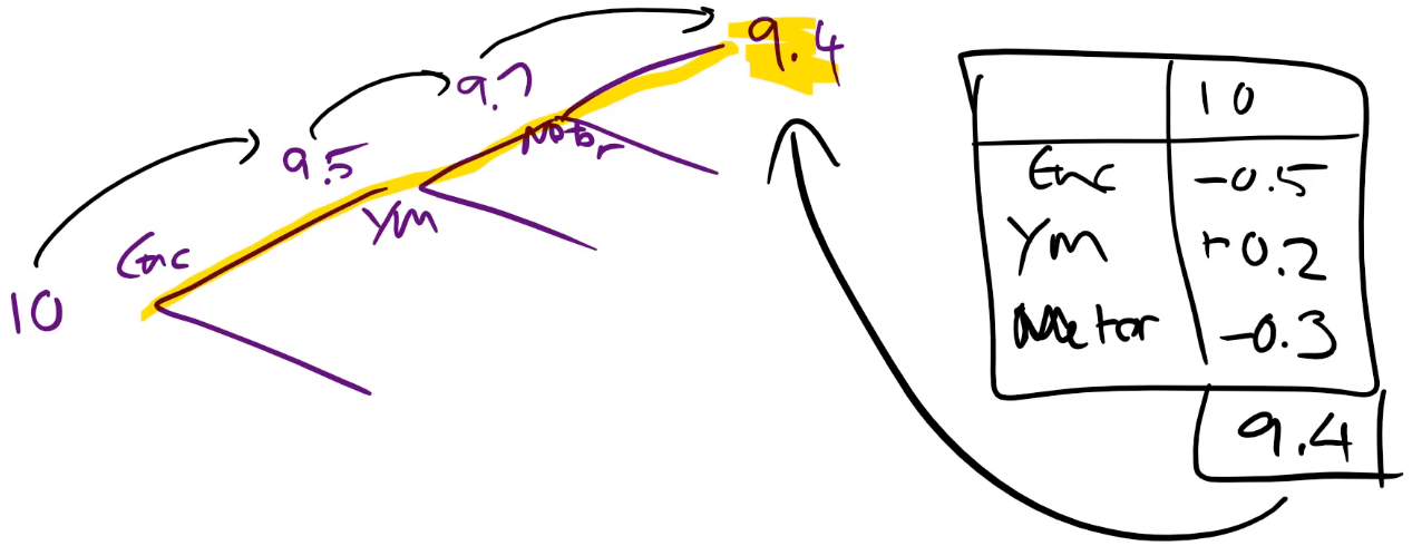
we call ti.predict and we get back the prediction of the price, the bias (i.e. the root of the tree — so this is just the average price for everybody so this is always going to be the same), and then the contributions which is how important is each of these things:
For example, at the very start, the average price was 10. Then we split on enclosure. For those with this enclosure, the average was 9.5. Then we split on year made less than 1990 and for those with that year made, the average price was 9.7. Then we split on the number of hours on the meter, and with this branch, we got 9.4.
from treeinterpreter import treeinterpreter as ti
df_train, df_valid = split_vals(df_raw[df_keep.columns], n_trn)
row = X_valid.values[None,0]; row
prediction, bias, contributions = ti.predict(m, row)
[o for o in zip(df_keep.columns[idxs], df_valid.iloc[0][idxs], contributions[0][idxs])]
8. important hyper parameters
-
- set_rf_samples
Determines how many rows are in each tree. So before we start a new tree, we either bootstrap a sample (i.e. sampling with replacement from the whole thing) or we pull out a subsample of a smaller number of rows and then we build a tree from there.
“We have a linear relationship between the number of leaf nodes and the size of the sample. So when you decrease the sample size, there are less final decisions that can be made. Therefore, the tree is going to be less rich in terms of what it can predict because it is making less different individual decisions and it also is making less binary choices to get to those decisions.”(https://medium.com/@hiromi_suenaga/machine-learning-1-lesson-4-a536f333b20d)
def set_rf_samples(n):
    """ Changes Scikit learn's random forests to give each tree a random sample of
    n random rows.
    """
    forest._generate_sample_indices = (lambda rs, n_samples:
        forest.check_random_state(rs).randint(0, n_samples, n))

def reset_rf_samples():
    """ Undoes the changes produced by set_rf_samples.
    """
    forest._generate_sample_indices = (lambda rs, n_samples:
        forest.check_random_state(rs).randint(0, n_samples, n_samples))
-
- min_samples_leaf
“Before, we assumed that min_samples_leaf=1, if it is set to 2, the new depth of the tree is log2(20000)-1. Each time we double the min_samples_leaf , we are removing one layer from the tree, and halving the number of leaf nodes (i.e. 10k). The result of increasing min_samples_leaf is that now each of our leaf nodes has more than one thing in, so we are going to get a more stable average that we are calculating in each tree. We have a little less depth (i.e. we have less decisions to make) and we have a smaller number of leaf nodes. So again, we would expect the result of that node would be that each estimator would be less predictive, but the estimators would be also less correlated. So this might help us avoid overfitting.” (https://medium.com/@hiromi_suenaga/machine-learning-1-lesson-4-a536f333b20d)
-
- max_features
“At each split, it will randomly sample columns (as opposed to set_rf_samples pick a subset of rows for each tree).
The overall effect of the max_features is the same — it’s going to mean that each individual tree is probably going to be less accurate but the trees are going to be more varied.
Particularly, if you were only doing a small number of trees (e.g. 10 trees) and you picked the same column set all the way through the tree, you are not really getting much variety in what kind of things it can find. So this way, at least in theory, seems to be something which is going to give us a better set of trees by picking a different random subset of features at every decision point.” (https://medium.com/@hiromi_suenaga/machine-learning-1-lesson-4-a536f333b20d)
9. extrapolition
This part was also new to me: RF has many good properties, but it is like “nearest neighbor” in tree space, so it cannot extrapolite well (cannot predict something haven’t seen).
Linear models are not flexible, but it can extrapolite.
10. data products
https://www.oreilly.com/radar/drivetrain-approach-data-products/
“data-train”
-
objective
-
levers: inputs we can control
-
data: think from first principles, what can help us identify … that can improve the outcome?
-
model:
e.g. how levers influence objective
e.g. target intervention for people with high predicted value